On September 1, 2022, The New York Times published a piece on opener popularity, including publishing the top 5 most popular openers. My analysis matches their actual data for the top 3! Pretty good for looking at tweets!
What are the most popular Wordle openers?
There has been a fair bit of analysis as to what is the best Wordle opener. However, how can can we figure out the most popular Twitter Wordle openers? I have attempted to do this by analyzing large samples of shared wordle scores on Twitter. Previously, I have used tweeted wordle scores to accurately predict the wordle solution for the day.
Analyzing the popularity of wordle openers based on shared scores is difficult, since on any given day all we know are the most popular opening patterns, e.g. 🟨🟩⬜⬜🟩. I use a Ridge linear regression to look for popular openers across 90 days, treating each possible opener as a feature/column. The words with the largest coefficients should be the most popular openers.
TDLR: the top 10 most common openers found through this method are below. This covers Wordles between and . Adieu is estimated at 4% of all openers. (Actual New York Times statistics place it at 5%)
The function make_first_guess_list creates a useful dataframe for analysis. It, and most other helper utilities are in the first_word.py file.
I start with the very useful kaggle data set wordle-tweets and extract directly from the zipfile which I download with the kaggle api. The get_first_words function processes the dataframe:
It removes tweeted scores that contain an invalid score line for that answer (likely played on a cached version of the puzzle, not the live one on the NY Times site).
It removes any tweets that have more than 6 score patterns.
It extracts the first pattern from the tweeted scores.
It maps on the answer for a given wordle id.
It groups by the answer for the day, and creates a dataframe that has score, target, guess, and some data on how popular that score is.
Colored squares are mapped to numbers. So a score of 🟨🟩⬜⬜🟩 becomes 12002.
Code
from first_word import make_first_guest_list,format_dfimport pandas as pdimport datetimewordle_start = datetime.datetime(2021, 6, 19)now = datetime.datetime.now()mapping_date_dict = {wordle_id: wordle_start+datetime.timedelta(days=wordle_id) for wordle_id inrange(210,500)}df = make_first_guest_list()format_df(df.sample(10))
Max wordle num 458
Filtered out 53709 of 983804 rows
score
target
guess
score_frequency_rank
score_count_fraction
wordle_num
guess_count
commonality
weighted_rank
00001
tiara
upper
13.0
0.022766
342
387
38341510
169.00
01000
badge
ceros
24.5
0.007752
321
666
0
600.25
00200
parer
corny
18.5
0.015355
454
269
378659
342.25
00000
girth
lemed
3.0
0.086652
355
3454
0
9.00
00000
alpha
texes
3.0
0.124421
451
4114
96227
9.00
00112
story
patsy
33.0
0.007643
317
32
1064602
1089.00
00000
doubt
pangs
1.0
0.213710
453
3684
194132
1.00
01021
egret
defer
52.5
0.002174
378
28
1207925
2756.25
00000
choke
buppy
4.0
0.097980
254
2791
0
16.00
01000
retro
bohos
10.0
0.032967
373
1066
0
100.00
Simple analysis
The large dataframe has one row for every pattern / guess / wordle answer combination. A simple way to look at common starter words would be to group by the opener and look which openers consistently rank high across several days.
This analysis leaves a lot to be desired. While other evidence indicates adieu is a popular opener, it does not seem like craze would be one. Plus, there are other words ending in -aze.
The 00000 all grey pattern is fairly common, so words with uncommon letters will show up a lot since 00000 is common because of the sheer volume of words that can create the pattern. So what happens if we filter out the null score?
The braze craze continues. Are people guessing braze regularly or is something else going on? BRAZE’s score line is common but what other words could make the same pattern?
Code
format_df(df.query('score == "00101" and wordle_num == 230').sort_values('commonality',ascending=False).head(10))
score
target
guess
score_frequency_rank
score_count_fraction
wordle_num
guess_count
commonality
weighted_rank
00101
pleat
image
9.0
0.029706
230
186
197874283
81.0
00101
pleat
share
9.0
0.029706
230
186
119294241
81.0
00101
pleat
until
9.0
0.029706
230
186
113090086
81.0
00101
pleat
grade
9.0
0.029706
230
186
54275130
81.0
00101
pleat
frame
9.0
0.029706
230
186
46079991
81.0
00101
pleat
usage
9.0
0.029706
230
186
25440406
81.0
00101
pleat
sharp
9.0
0.029706
230
186
24904199
81.0
00101
pleat
grace
9.0
0.029706
230
186
17642126
81.0
00101
pleat
villa
9.0
0.029706
230
186
17587586
81.0
00101
pleat
solve
9.0
0.029706
230
186
13452150
81.0
There are many other words that make the same pattern. BRAZE could be popular or perhaps it is riding the coattails of some other _RA_E word?
Linear Regression
A better approach is to control for the presence of other words. If BRAZE only does well when it’s paired with GRACE or GRADE or SHARE than a linear regression should isolate the guesses that actually are predictive of a popular score count line. Since I’m trying to account for colinearity, I will use a Ridge regression.
One difficulty came from getting the dataframe into the right format. I want one row per wordle number / score pattern, with each possible guess a column of 1 or 0. The “dependent” is the fraction of all tweeted opening score patterns that match that pattern. (e.g. for wordle 230 what fraction of all tweeted scores started 🟨🟩⬜⬜🟨). Another feature is the number of words that could produce that pattern.
I normalize the data somewhat, and then fit a model across all the word features as well as guess count. The Ridge helps control the size of the coefficients, and is neccessary to handle the colinearity of the variables.
Code
df.rename(columns={'score': 'score_pattern'}, inplace=True)one_hot_encoded_data = pd.crosstab( [df['wordle_num'], df['score_pattern']], df['guess']).join( df.groupby(['wordle_num','score_pattern'])[['score_count_fraction','guess_count']].first()).reset_index()one_hot_encoded_data.dropna(subset=['score_count_fraction'],inplace=True) #don't need patterns no one actually guessed# actually not sure if fillna 0 would be better?std = one_hot_encoded_data['score_count_fraction'].std()one_hot_encoded_data['guess_count_orig'] = one_hot_encoded_data['guess_count']guess_count_std = one_hot_encoded_data['guess_count'].std()guess_count_mean = one_hot_encoded_data['guess_count'].mean()one_hot_encoded_data['guess_count'] = (one_hot_encoded_data['guess_count'] - guess_count_mean ) / guess_count_std
Fitting the Ridge model to the 90 most recent wordles.
Code
from sklearn import linear_modelfrom tweet_script import today_wordle_numlookback_num = today_wordle_num() -90data = one_hot_encoded_data.query("wordle_num != 258 and wordle_num > @lookback_num ") #explained further down, this data point has particularly bad colinearity issuesend_date = mapping_date_dict[data['wordle_num'].max()].strftime("%B %-d, %Y")begin_date = mapping_date_dict[data['wordle_num'].min()].strftime("%B %-d, %Y")X= data.drop( columns=[ 'score_count_fraction', 'wordle_num','score_pattern','guess_count_orig'],errors='ignore') # fit to the one hot encoded guesses and the total guess county=data['score_count_fraction'] # our dependent is the fraction of guesses that had the score patternr = linear_model.RidgeCV(alphas=[5,10,15])r.fit(X,y)r.alpha_
RidgeCV(alphas=[5, 10, 15])
In a Jupyter environment, please rerun this cell to show the HTML representation or trust the notebook. On GitHub, the HTML representation is unable to render, please try loading this page with nbviewer.org.
RidgeCV(alphas=[5, 10, 15])
5
Results!
Now we can look at the variable coefficients to see which words most strongly predict a popular pattern. The top few guesses contain somefamiliar choices.
Ok, so adieu is popular but exactly how many people are actually using it every day? Below, I look at what fraction of all tweeted score patterns are consistent with adieu and plot that against how many other words could have also made that pattern.
So in the data for adieu, the minimum fraction that could be adieu was about 6% (Wordle 206), with Wordle 344 indicating maybe as high as 7.5%.
However, I have the fitted Ridge model, and I can use it to predict what adieu (and all the other top choices) would do with a guess count of 1 and where adieu was the only word that could make it. (Which I believe is the same as the the coefficient plus the intercept.)
Code
series_list = []for word in top_openers['variable'].head(15): predict_dict = {word:1,'guess_count':(1- guess_count_mean) / guess_count_std} series_list.append(pd.Series({x:predict_dict.get(x,int(0)) for x in X.columns}))predict_on_this = pd.DataFrame(series_list)top_15 = top_openers.head(15).reset_index(drop=True)top_15.loc[:,'estimated_fraction'] = r.predict(predict_on_this)format_df(top_15.reset_index(),formatters={'estimated_fraction':'{:,.2%}'.format})
index
variable
coef
estimated_fraction
0
adieu
0.039502
4.02%
1
audio
0.014438
1.52%
2
stare
0.013428
1.42%
3
irate
0.010029
1.08%
4
raise
0.009542
1.03%
5
great
0.007361
0.81%
6
arise
0.006987
0.77%
7
crate
0.005715
0.64%
8
steam
0.005546
0.63%
9
train
0.005466
0.62%
10
crane
0.005010
0.57%
11
arose
0.004998
0.57%
12
amies
0.004935
0.57%
13
ajies
0.004854
0.56%
14
soare
0.004568
0.53%
This indicates that adieu represents about 4.02% of all starters. This is considerably lower than looking at the score count fraction graph. The Ridge model does seem to find the correct top openers, but is performing poorly at the actual frequency of the most common openers, and at predicting the score when the total number of guesses that can make a pattern approaches 1.
From additional inspection of the errors, I would say the model is off by almost a factor of two when estimating the commonality of the most common openers.
On February 6, 3Blue1Brown released a video positing that CRANE was the best opener. Though this was later recanted, it generated plenty of mediacoverage. CRANE was high on my list based on recent wordles, how does it look before the video?
Code
data_past = one_hot_encoded_data.query('wordle_num <= 232')X= data_past.drop( columns=[ 'score_count_fraction', 'wordle_num']) # fit to the one hot encouded guesses and the total guess county=data_past['score_count_fraction'] # our dependent is the fraction of guesses that had the score patternr = linear_model.Ridge(alpha=10)r.fit(X,y)out = pd.DataFrame(list(zip(r.coef_, r.feature_names_in_)), columns=['coef', 'variable']).sort_values('coef',ascending=False)out['guess_rank'] = out['coef'].rank(ascending=False)format_df(out.query('variable == "crane"'))
Ridge(alpha=10)
In a Jupyter environment, please rerun this cell to show the HTML representation or trust the notebook. On GitHub, the HTML representation is unable to render, please try loading this page with nbviewer.org.
Ridge(alpha=10)
coef
variable
guess_rank
0.000294
crane
1022.0
Prior to Wordle 233, CRANE ranked 1018! Quite the turnaround. (Alpha values may not be optimal for these smaller sample sizes) You can see this even in the cruder analysis, where the ranks for CRANE were much lower in the past.
---title: "Most Popular Wordle Openers"format: html: code-fold: true code-tools: true toc: true toc-depth: 4 toc-location: left output-file: index.htmljupyter: python3execute: cache: true---## Preface[Back to All Projects page](https://marcoshuerta.com/projects.html)[Twitterwordle Github Repository](https://github.com/astrowonk/TwitterWordle)_This is a [Quarto](https://quarto.org) version of [my original jupyter notebook](https://github.com/astrowonk/TwitterWordle/blob/main/Popular%20Wordle%20Openers.ipynb). I plan to update this version regularly. See the [quarto .qmd source on Github here](https://github.com/astrowonk/TwitterWordle/blob/main/openers.qmd).__On September 1, 2022, The New York Times [published a piece](https://www.nytimes.com/2022/09/01/crosswords/wordle-starting-words-adieu.html) on opener popularity, including publishing the top 5 most popular openers. My analysis matches their actual data for the top 3! Pretty good for looking at tweets!_## What are the most popular Wordle openers? There has been a fair bit of analysis as to what is the best Wordle opener. However, how can can we figure out the most _popular_ Twitter Wordle openers? I have attempted to do this by analyzing large samples of shared wordle scores on Twitter. Previously, I have used tweeted wordle scores to [accurately predict](https://twitter.com/thewordlebot/status/1498661373626265600) the wordle solution for the day.Analyzing the popularity of wordle openers based on shared scores is difficult, since on any given day all we know are the most popular opening _patterns_, e.g. `🟨🟩⬜⬜🟩`. I use a Ridge linear regression to look for popular openers across 90 days, treating each possible opener as a feature/column. The words with the largest coefficients should be the most popular openers. TDLR: the top 10 most common openers found through this method are below. This covers Wordles between <strong> ${the_dates[0]} </strong> and <strong> ${the_dates[1]} </strong>. `Adieu` is estimated at 4% of all openers. (Actual New York Times statistics place it at 5%)1. ${my_output[0]}2. ${my_output[1]} 3. ${my_output[2]}4. ${my_output[3]}5. ${my_output[4]}6. ${my_output[5]}7. ${my_output[6]}8. ${my_output[7]}9. ${my_output[8]}10. ${my_output[9]}The top three of the list above are the same as New York Times' own data [written up on September 1.](https://www.nytimes.com/2022/09/01/crosswords/wordle-starting-words-adieu.html). 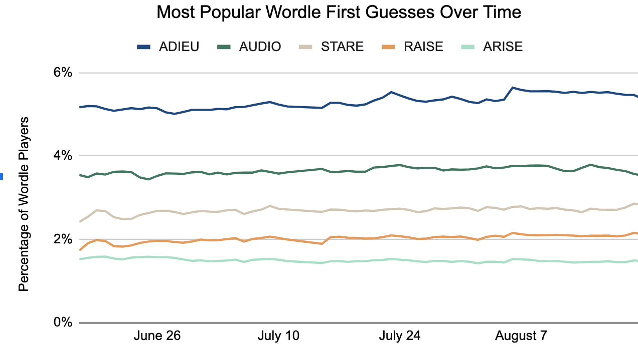## Load and prep the dataThe function `make_first_guess_list` creates a useful dataframe for analysis. It, and most other helper utilities are in the [first_word.py](https://github.com/astrowonk/TwitterWordle/blob/main/first_word.py) file.I start with the very useful kaggle data set [wordle-tweets](https://www.kaggle.com/benhamner/wordle-tweets) and extract directly from the zipfile which I download with the [kaggle api](https://github.com/Kaggle/kaggle-api). The `get_first_words` function processes the dataframe:1. It removes tweeted scores that contain an invalid score line for that answer (likely played on a cached version of the puzzle, not the live one on the NY Times site).2. It removes any tweets that have more than 6 score patterns.3. It extracts the first pattern from the tweeted scores.4. It maps on the answer for a given wordle id.5. It groups by the answer for the day, and creates a dataframe that has score, target, guess, and some data on how popular that score is.6. Colored squares are mapped to numbers. So a score of `🟨🟩⬜⬜🟩` becomes `12002`.```{python}from first_word import make_first_guest_list,format_dfimport pandas as pdimport datetimewordle_start = datetime.datetime(2021, 6, 19)now = datetime.datetime.now()mapping_date_dict = {wordle_id: wordle_start+datetime.timedelta(days=wordle_id) for wordle_id inrange(210,500)}df = make_first_guest_list()format_df(df.sample(10))```## Simple analysisThe large dataframe has one row for every pattern / guess / wordle answer combination. A simple way to look at common starter words would be to group by the opener and look which openers consistently rank high across several days.```{python}df.groupby('guess')['score_frequency_rank'].mean().sort_values().head(10)```This analysis leaves a lot to be desired. While other evidence indicates `adieu` is a popular opener, it does not seem like `craze` would be one. Plus, there are other words ending in `-aze`.The `00000` all grey pattern is fairly common, so words with uncommon letters will show up a lot since `00000` is common because of the sheer volume of words that can create the pattern. So what happens if we filter out the null score? ```{python}df.query("score != '00000'").groupby('guess')['score_frequency_rank'].mean().sort_values().head(10)```The braze craze continues. Are people guessing `braze` regularly or is something else going on? BRAZE's score line is common but what other words could make the same pattern? ```{python}format_df(df.query('score == "00101" and wordle_num == 230').sort_values('commonality',ascending=False).head(10))```There are many other words that make the same pattern. `BRAZE` could be popular or perhaps it is riding the coattails of some other `_RA_E` word?## Linear RegressionA better approach is to control for the presence of other words. If BRAZE only does well when it's paired with GRACE or GRADE or SHARE than a linear regression should isolate the guesses that actually are predictive of a popular score count line. Since I'm trying to account for colinearity, I will use a Ridge regression.One difficulty came from getting the dataframe into the right format. I want one row per wordle number / score pattern, with each possible guess a column of 1 or 0. The "dependent" is the fraction of all tweeted opening score patterns that match that pattern. (e.g. for wordle 230 what fraction of all tweeted scores started `🟨🟩⬜⬜🟨`). Another feature is the number of words that could produce that pattern.I discovered [pd.crosstab](https://pandas.pydata.org/docs/reference/api/pandas.crosstab.html), and there are [other methods that were all better](https://stackoverflow.com/questions/46791626/one-hot-encoding-multi-level-column-data) than what I had been doing originally (an awful groupby loop than took over a minute.)I normalize the data somewhat, and then fit a model across all the word features as well as guess count. The [Ridge](https://scikit-learn.org/stable/modules/linear_model.html#ridge-regression-and-classification) helps control the size of the coefficients, and is neccessary to handle the colinearity of the variables.```{python}df.rename(columns={'score': 'score_pattern'}, inplace=True)one_hot_encoded_data = pd.crosstab( [df['wordle_num'], df['score_pattern']], df['guess']).join( df.groupby(['wordle_num','score_pattern'])[['score_count_fraction','guess_count']].first()).reset_index()one_hot_encoded_data.dropna(subset=['score_count_fraction'],inplace=True) #don't need patterns no one actually guessed# actually not sure if fillna 0 would be better?std = one_hot_encoded_data['score_count_fraction'].std()one_hot_encoded_data['guess_count_orig'] = one_hot_encoded_data['guess_count']guess_count_std = one_hot_encoded_data['guess_count'].std()guess_count_mean = one_hot_encoded_data['guess_count'].mean()one_hot_encoded_data['guess_count'] = (one_hot_encoded_data['guess_count'] - guess_count_mean ) / guess_count_std```Fitting the Ridge model to the 90 most recent wordles.```{python}from sklearn import linear_modelfrom tweet_script import today_wordle_numlookback_num = today_wordle_num() -90data = one_hot_encoded_data.query("wordle_num != 258 and wordle_num > @lookback_num ") #explained further down, this data point has particularly bad colinearity issuesend_date = mapping_date_dict[data['wordle_num'].max()].strftime("%B %-d, %Y")begin_date = mapping_date_dict[data['wordle_num'].min()].strftime("%B %-d, %Y")X= data.drop( columns=[ 'score_count_fraction', 'wordle_num','score_pattern','guess_count_orig'],errors='ignore') # fit to the one hot encoded guesses and the total guess county=data['score_count_fraction'] # our dependent is the fraction of guesses that had the score patternr = linear_model.RidgeCV(alphas=[5,10,15])r.fit(X,y)r.alpha_```### Results!Now we can look at the variable coefficients to see which words most strongly predict a popular pattern. The top few guesses contain [some](https://yougov.co.uk/topics/entertainment/articles-reports/2022/02/03/wordle-starter-words-hard-mode-and-x6-how-are-brit)[familiar](https://today.yougov.com/topics/lifestyle/articles-reports/2022/02/18/wordle-willingness-to-pay-poll) choices. ```{python}from IPython.display import display, HTMLtop_openers = pd.DataFrame(list(zip(r.feature_names_in_,r.coef_)), columns=['variable', 'coef']).sort_values('coef',ascending=False)display(HTML(top_openers.head(15).to_html(index=False)))top_openers_list = top_openers.query('variable != "guess_count"')['variable'].head(15).tolist()``````{python}#| echo: false#| warning: false#| error: false#| output: falseojs_define(my_output = top_openers_list)ojs_define(the_dates = [begin_date,end_date])```### Just how popular is _adieu_?Ok, so _adieu_ is popular but exactly how many people are actually using it every day? Below, I look at what fraction of all tweeted score patterns are consistent with `adieu` and plot that against how many *other* words could have also made that pattern.```{python}guess ='adieu'df.query(f'guess == @guess and guess_count < 400 and wordle_num > @lookback_num').sort_values('wordle_num').plot.scatter( x='guess_count', y='score_count_fraction', hover_data=['score_pattern', 'wordle_num'],# color='guess_count', title=f'{guess.upper()} popularity', backend='plotly',# color_continuous_scale='bluered', )```So in the data for `adieu`, the minimum fraction that could be `adieu` was about 6% (Wordle 206), with Wordle 344 indicating maybe as high as 7.5%. However, I have the fitted Ridge model, and I can use it to predict what `adieu` (and all the other top choices) would do with a guess count of 1 and where `adieu` was the only word that could make it. (Which I believe is the same as the the coefficient plus the intercept.)```{python}series_list = []for word in top_openers['variable'].head(15): predict_dict = {word:1,'guess_count':(1- guess_count_mean) / guess_count_std} series_list.append(pd.Series({x:predict_dict.get(x,int(0)) for x in X.columns}))predict_on_this = pd.DataFrame(series_list)top_15 = top_openers.head(15).reset_index(drop=True)top_15.loc[:,'estimated_fraction'] = r.predict(predict_on_this)format_df(top_15.reset_index(),formatters={'estimated_fraction':'{:,.2%}'.format})``````{python}#| echo: falsefrom IPython.display import display, Markdowndisplay(Markdown(f"""This indicates that `adieu` represents about {top_15['estimated_fraction'].iloc[0]:.2%} of all starters. This is considerably lower than looking at the score count fraction graph. The Ridge model does seem to find the correct top openers, but is performing poorly at the actual frequency of the most common openers, and at predicting the score when the total number of guesses that can make a pattern approaches 1."""))```From additional inspection of the errors, I would say the model is off by almost a factor of two when estimating the commonality of the most common openers.```{python}new_df = X.copy()new_df['predicted_score_count_fraction'] = r.predict(X)new_df = new_df.join(data[['score_count_fraction', 'wordle_num', 'score_pattern', 'guess_count_orig']])new_df['score_count_error'] = ( new_df['score_count_fraction'] - new_df['predicted_score_count_fraction']) / new_df['score_count_fraction']new_df.query('guess_count_orig < 20 and score_count_fraction > .01').plot.scatter( x='guess_count_orig', y='score_count_error', trendline='ols', labels={'score_count_error':'Score Count Error (Fractional)','guess_count_orig': "Guess Count" }, hover_data={'score_pattern': True,'wordle_num': True,'predicted_score_count_fraction': ':.3f','score_count_fraction': ':.3f','score_count_error': ':.4f' }, )```## CRANEOn February 6, 3Blue1Brown released a video positing that [CRANE was the best opener](https://www.youtube.com/watch?v=v68zYyaEmEA). Though this was later [recanted](https://www.youtube.com/watch?v=fRed0Xmc2Wg), it generated plenty of [media](https://kotaku.com/wordle-starting-word-math-science-bot-algorithm-crane-p-1848496404)[coverage](https://www.forbes.com/sites/paultassi/2022/02/08/the-best-wordle-starter-word-a-first-guess-through-science/?sh=94c150a27909). CRANE was high on my list based on recent wordles, how does it look before the video?```{python}data_past = one_hot_encoded_data.query('wordle_num <= 232')X= data_past.drop( columns=[ 'score_count_fraction', 'wordle_num']) # fit to the one hot encouded guesses and the total guess county=data_past['score_count_fraction'] # our dependent is the fraction of guesses that had the score patternr = linear_model.Ridge(alpha=10)r.fit(X,y)out = pd.DataFrame(list(zip(r.coef_, r.feature_names_in_)), columns=['coef', 'variable']).sort_values('coef',ascending=False)out['guess_rank'] = out['coef'].rank(ascending=False)format_df(out.query('variable == "crane"'))```Prior to Wordle 233, CRANE ranked 1018! Quite the turnaround. (Alpha values may not be optimal for these smaller sample sizes) You can see this even in the cruder analysis, where the ranks for CRANE were much lower in the past.```{python}guess ='crane'myplot = df.query(f'guess == @guess').sort_values('wordle_num').plot.scatter( x='wordle_num', y='score_frequency_rank', color='guess_count', title=f'{guess.upper()} popularity',backend='plotly', color_continuous_scale='bluered', )myplot.update_yaxes(autorange="reversed")```[Back to All Projects page](https://marcoshuerta.com/projects.html)[Twitterwordle Github Repository](https://github.com/astrowonk/TwitterWordle)```{ojs}//| code-fold: false//| echo: false//| output: falseviewof something =1```
